
Back in Excel Interface Explained: Ribbon, Toolbar, and Backstage View for Beginners, I showed you the Ribbon, the Quick Access Toolbar, and Backstage View. Now it’s time to zoom into one tab at a time, starting with the one you’ll use the most. This is the Excel Home tab, fully explained, command by command.
Quick Takeaway: The Home tab holds your everyday formatting and editing tools. Think bold text, cell colors, number formats, sorting, and AutoSum. It’s split into seven groups: Clipboard, Font, Alignment, Number, Styles, Cells, and Editing. You’ll live on this tab more than any other.
This post breaks down every command sitting on it, what each one actually does, its shortcut if it has one, and when you’d reach for it.
By the end, you won’t just recognize these buttons. You’ll know exactly which one to click, and why.
A quick note on versions: Every command below applies to Excel 2016 and later, Microsoft 365, Excel for Mac, and Excel for the web.
Group 1: Clipboard
This tiny group on the far left does more heavy lifting than its size suggests.
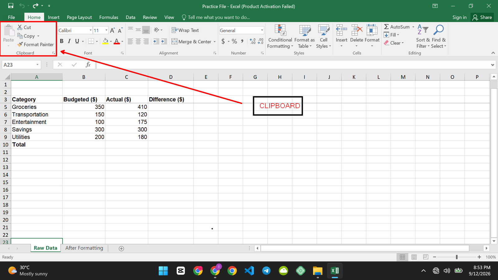
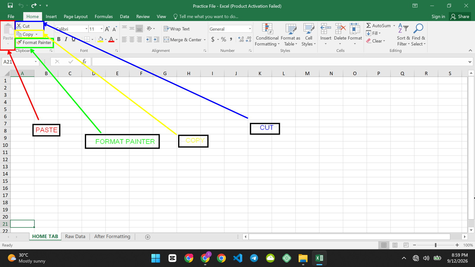
Paste: It drops whatever you last copied or cut into the selected cell.
Shortcut: Ctrl+V.
Use case: you’ll use this dozens of times a day, it’s the most-used command on the whole Ribbon.
Cut: It grabs the selected cell’s content and removes it, ready to paste elsewhere.
Shortcut: Ctrl+X.
Use case: moving a row of data to a new spot without leaving a duplicate behind.
Copy: It grabs the selected cell’s content without removing it.
Shortcut: Ctrl+C.
Use case: duplicating a formula or a formatted cell somewhere else in your sheet.
Format Painter: It copies formatting only, not the data, from one cell and applies it to another.
Shortcut: no default shortcut, but you can access it with Alt, H, F, P.
Use case: you’ve formatted one header cell exactly how you want it, and now you need five more headers to match. Click the cell, click Format Painter, then click the next cell.
Group 2: Font
This is where you make your text look the way you want it to look.
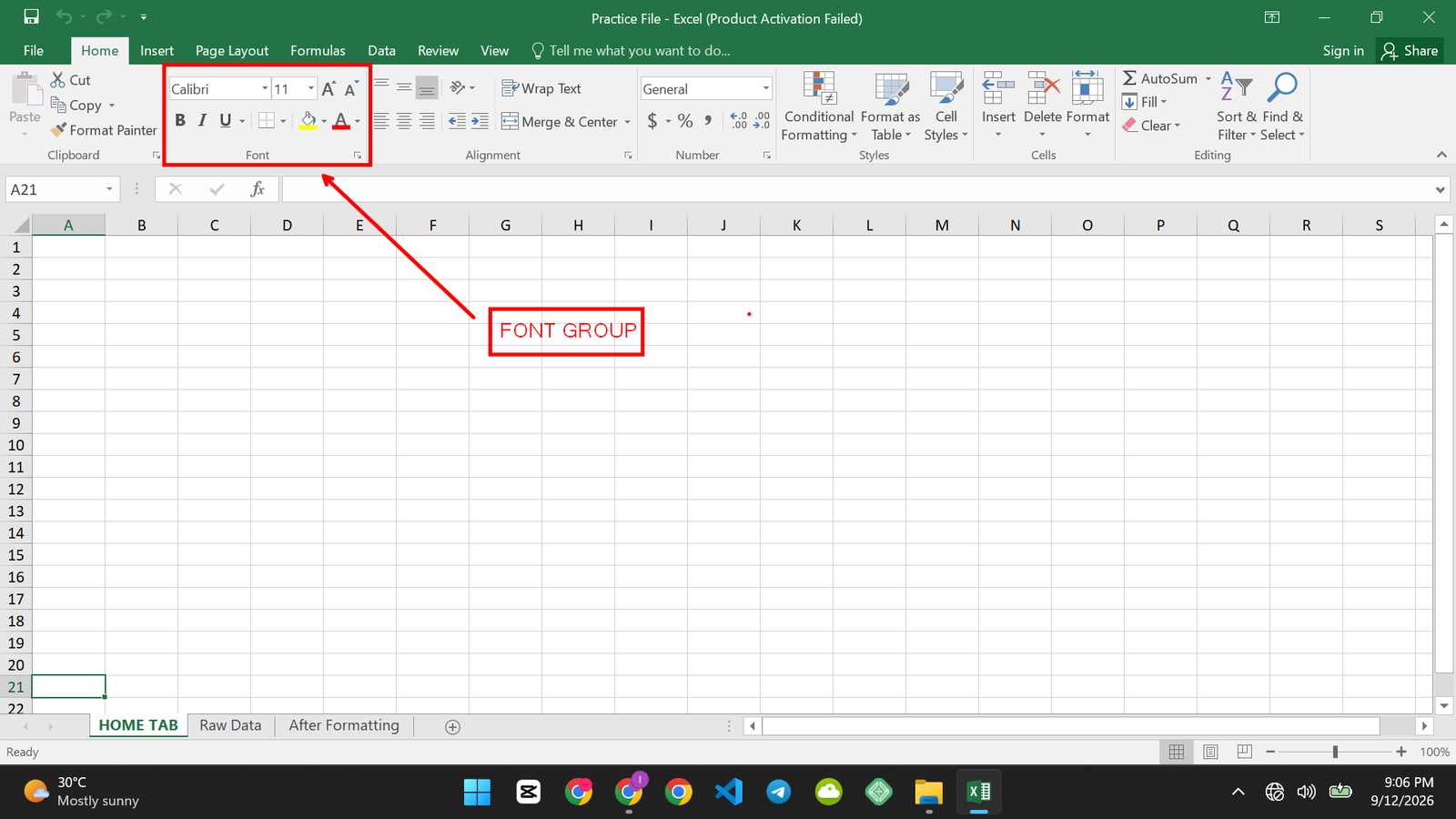
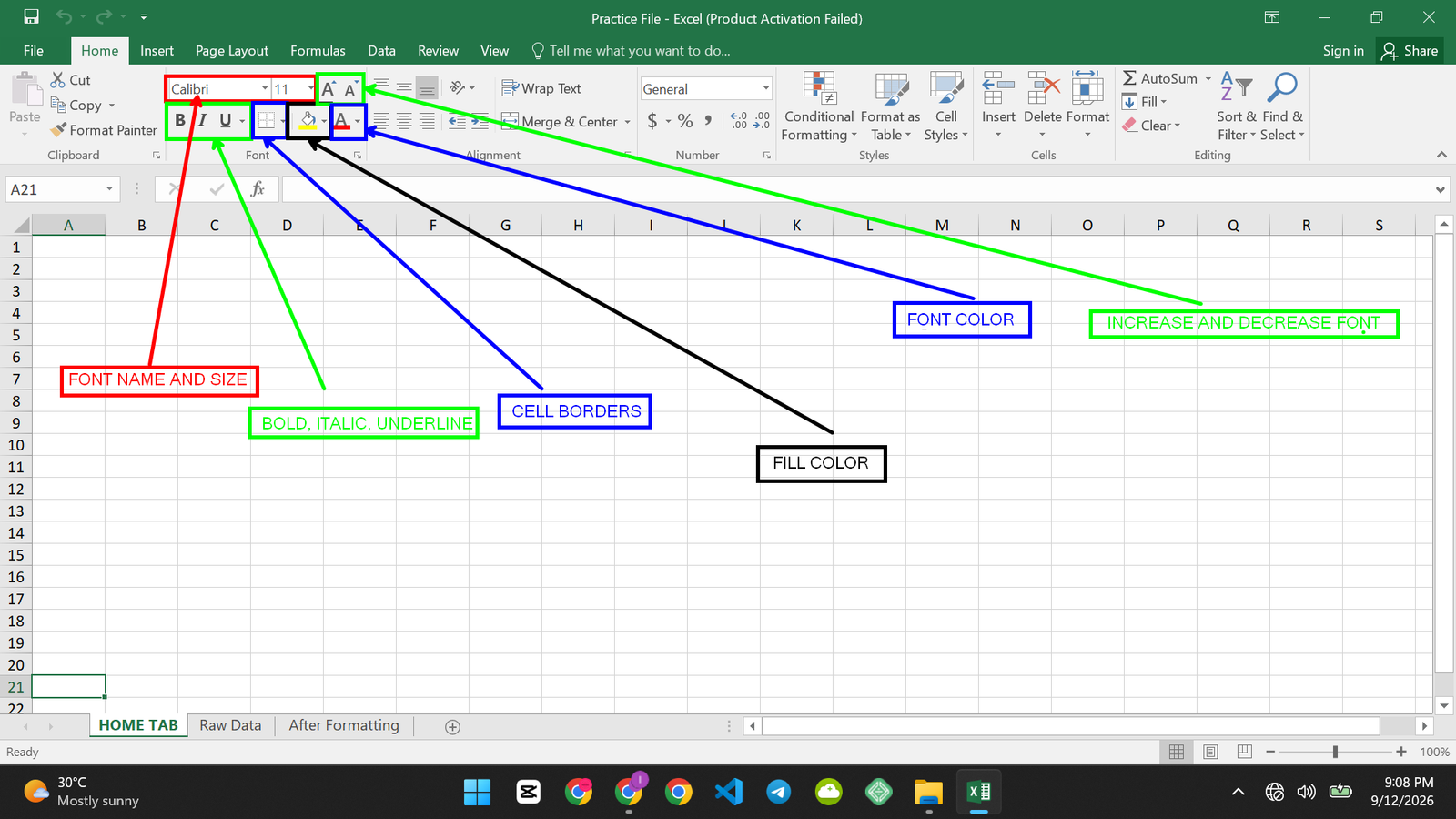
Font Name and Font Size: It changes the typeface and the size of the selected text.
Shortcut: no default shortcut, use the dropdowns.
Use case: matching your company’s brand font, or making a title stand out.
Bold, Italic, Underline: It exactly what it says, adds emphasis to selected text.
Shortcut: Ctrl+B for bold, Ctrl+I for italic, Ctrl+U for underline.
Use case: bolding your header row so it’s obvious at a glance where your data starts.
Borders: It adds lines around or inside selected cells.
Shortcut: no simple default, but Ctrl+Shift+& adds an outline border and Ctrl+Shift+_ removes it. Use case: separating a total row from the data above it.
Fill Color: It shades the background of selected cells.
Shortcut: no default shortcut.
Use case: highlighting a category, or shading alternating rows for readability.
Font Color: It changes the color of selected text.
Shortcut: no default shortcut.
Use case: making negative numbers red, though conditional formatting handles this automatically and I’d usually pick that instead.
Increase Font Size: It makes your font bigger with each click.
Decrease Font Size: It makes your font smaller with each click.
Use case for the above two(2): This is useful when you don’t have a font size beforehand and you’re just doing trial and error to see which font size fits better.
Group 3: Alignment
This group controls where your content sits inside a cell.
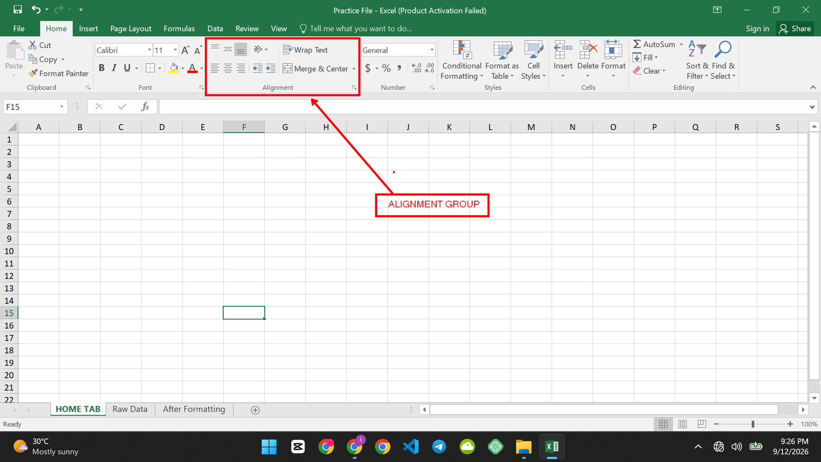
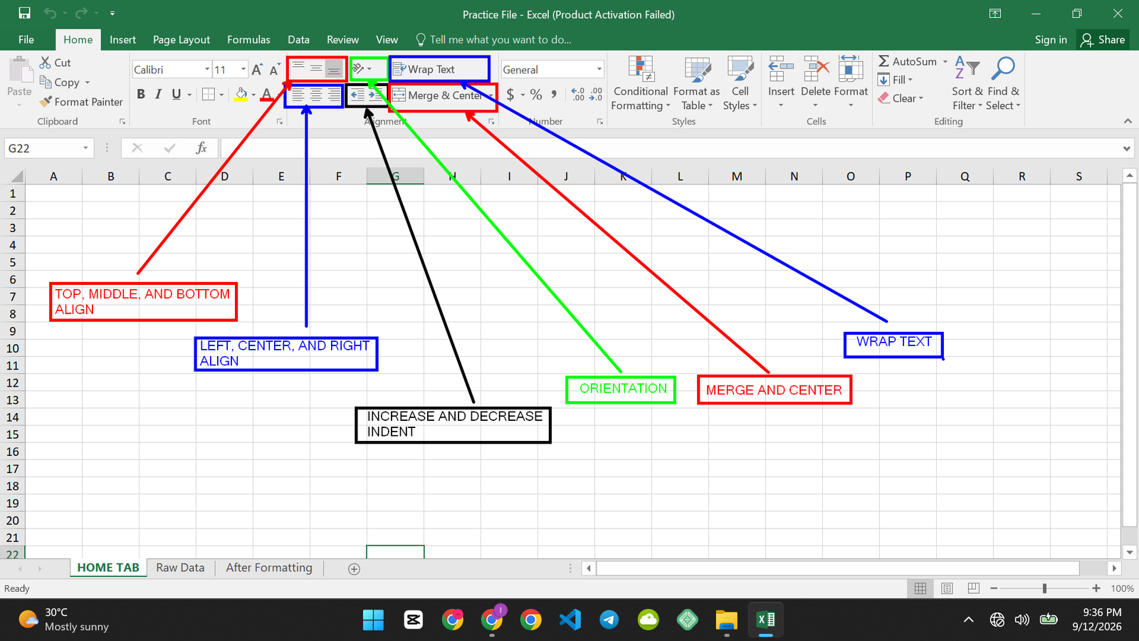
Top, Middle, Bottom Align: It positions text vertically within a cell.
Shortcut: no default shortcut.
Use case: centering text in a taller row so it doesn’t look stuck to the top.
Left, Center, Right Align: It positions text horizontally within a cell.
Shortcut: no default shortcut.
Use case: centering column headers over the data beneath them.
Orientation: It angles or rotates text inside a cell.
Shortcut: no default shortcut.
Use case: fitting a long column header into a narrow column by angling the text.
Wrap Text: It forces long text to wrap onto multiple lines instead of spilling into the next cell. Shortcut: no default shortcut.
Use case: a cell with a full sentence of notes that you want fully visible without widening the column.
Merge & Center: It combines selected cells into one and centers the content across them. Shortcut: no default shortcut.
Use case: a title that should span across several columns, like “My Monthly Budget Tracker”
Increase and Decrease Indent: It pushes cell content inward or pulls it back, in small steps. Shortcut: no default shortcut.
Use case: nesting sub-items under a main category so the hierarchy is visible at a glance.
Group 4: Number
This is where your raw numbers turn into numbers that mean something.
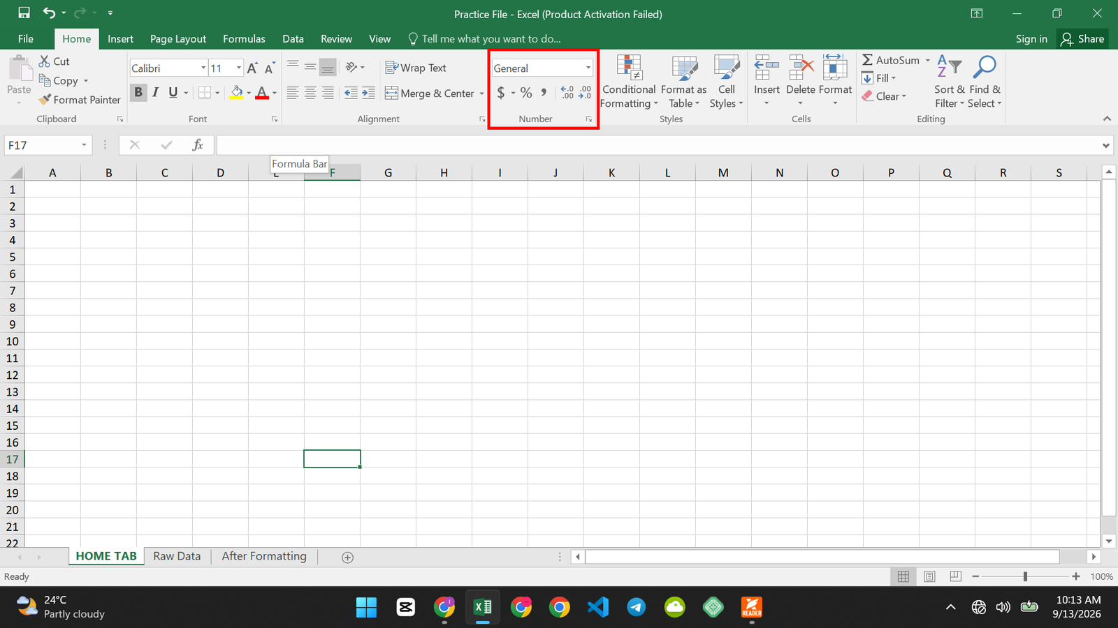
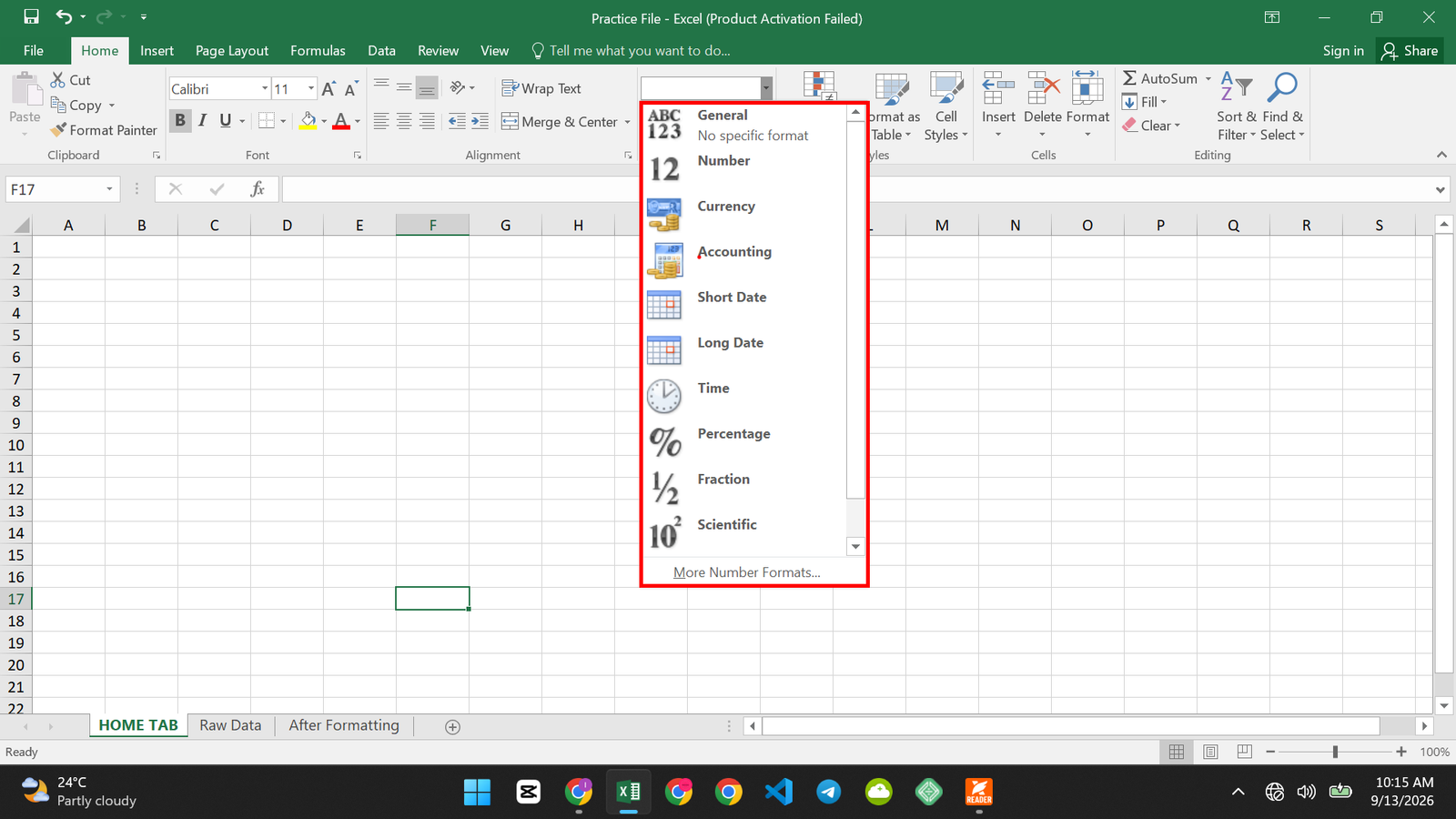
Number Format Dropdown: It lets you pick how a number displays: general, currency, date, percentage, and more.
Shortcut: no default shortcut for the dropdown itself.
Use case: turning a plain “45658” into a readable date, or “0.15” into “15%.”
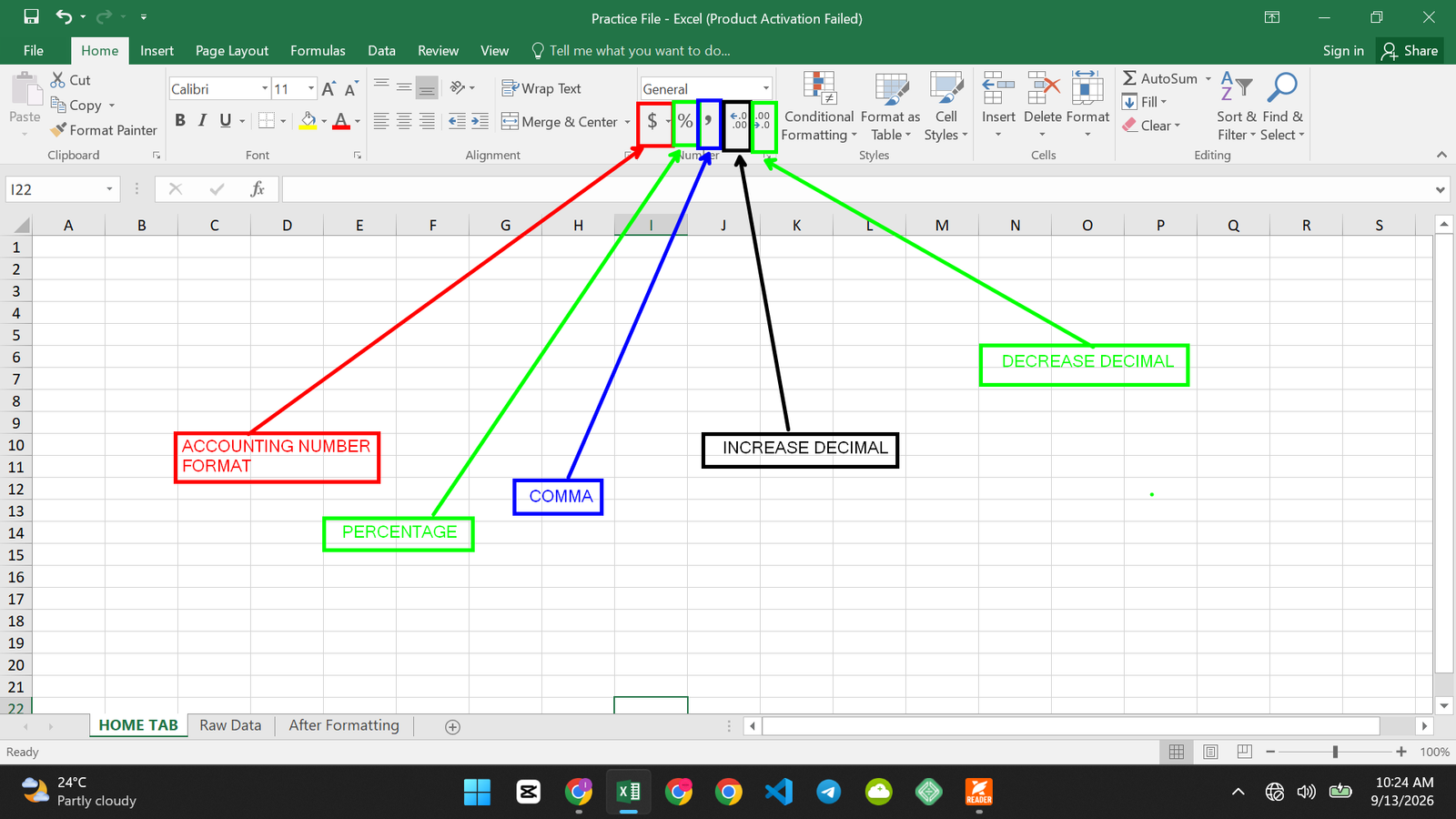
Accounting Number Format: It adds a currency symbol and aligns decimal points down a column.
Shortcut: Ctrl+Shift+$ (also written as Ctrl+Shift+4).
Use case: formatting currency amounts so they read like real dollar amounts instead of plain numbers.
Percent Style: It multiplies the number by 100 and adds a percent sign.
Shortcut: Ctrl+Shift+% (also written as Ctrl+Shift+5).
Comma Style: It adds a thousands separator, without a currency symbol.
Shortcut: Ctrl+Shift+! (also written as Ctrl+Shift+1).
Use case: large numbers that are easier to read with commas. E.g, 100000 becomes 100,000.
Increase and Decrease Decimal: It adds or removes one decimal place at a time.
Shortcut: no default shortcut.
Use case: trimming a formula result like 410.33333 down to a clean 410.33.
Group 5: Styles
This group applies pre-built looks instead of formatting cells one at a time.
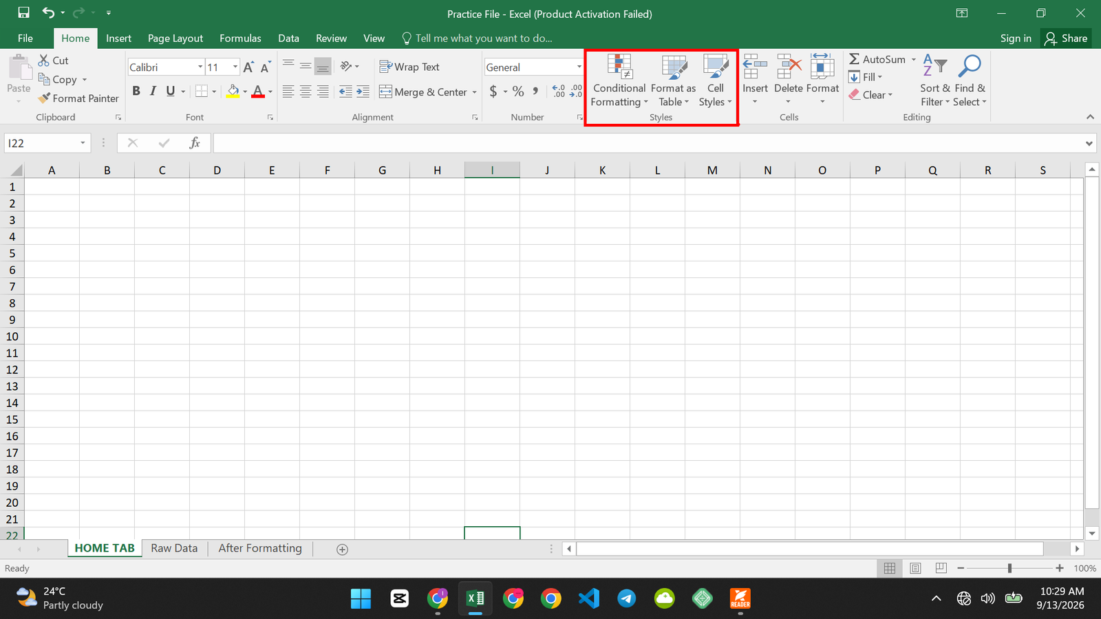
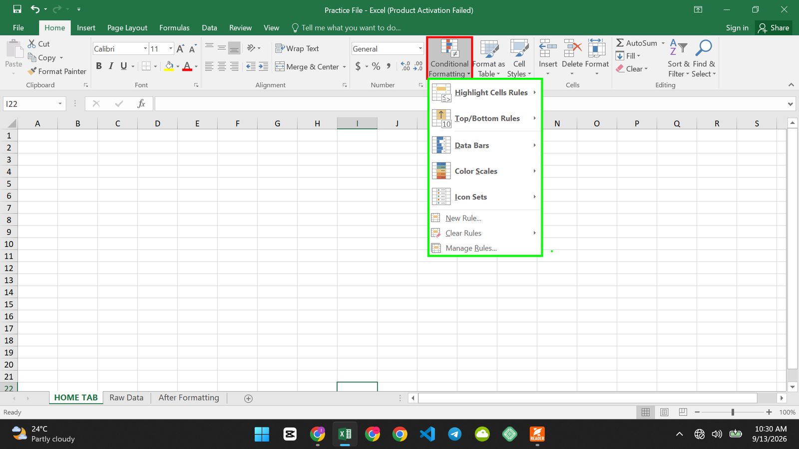
Conditional Formatting: It automatically changes how a cell looks based on its value.
Shortcut: no default shortcut.
Use case: Use rules to identify cells with certain characteristics in a range.
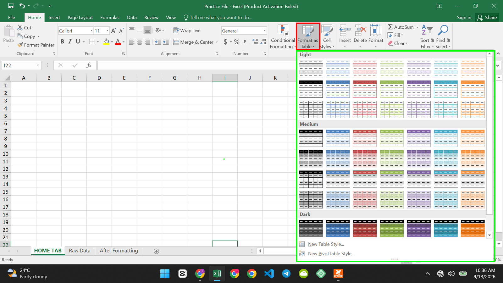
Format as Table: It turns a plain range into a structured table with filter buttons and banded rows.
Shortcut: Ctrl+T.
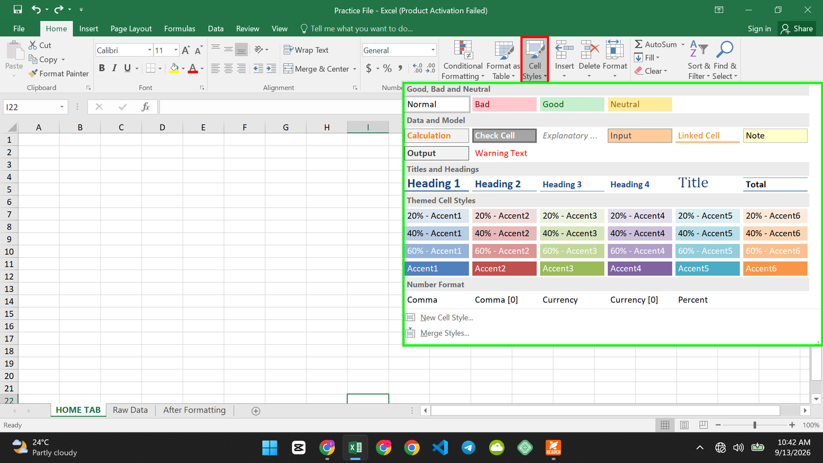
Cell Styles: It applies a saved combination of font, color, and border settings in one click. Shortcut: no default shortcut.
Use case: quickly marking a cell as a “Warning” or “Good” style without picking each format separately.
Group 6: Cells
This group changes the structure of your sheet, not just the formatting.
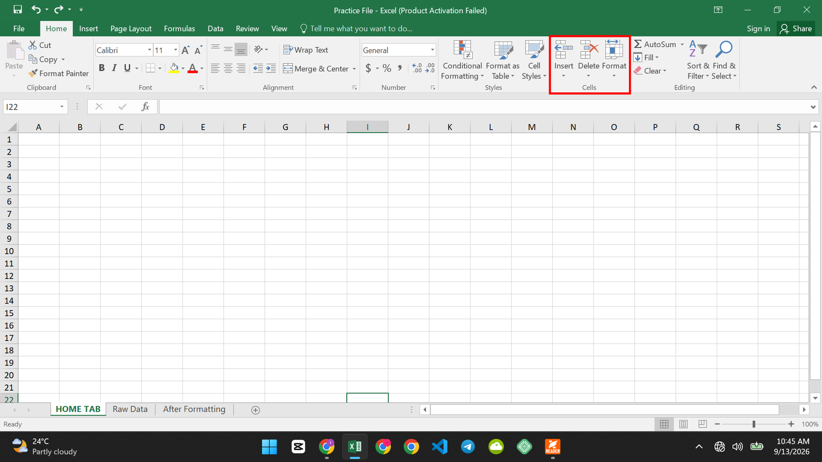
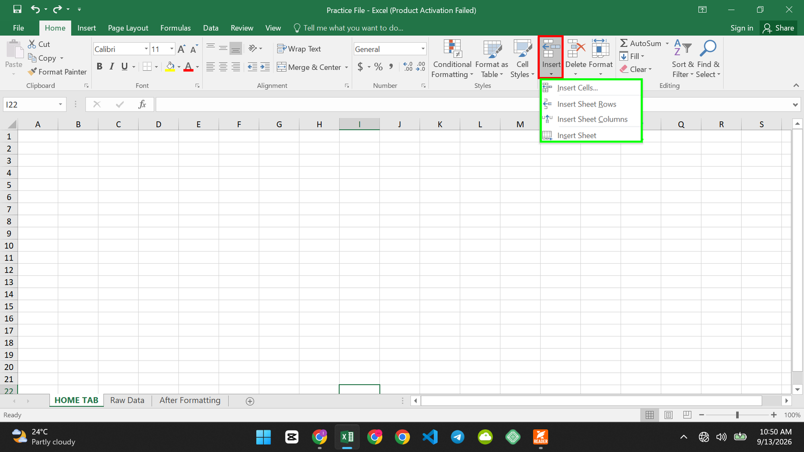
Insert: It adds a new cell, row, column, or sheet.
Shortcut: Ctrl+Shift+= (plus sign).
Use case: Use to slot a new row in without overwriting anything.
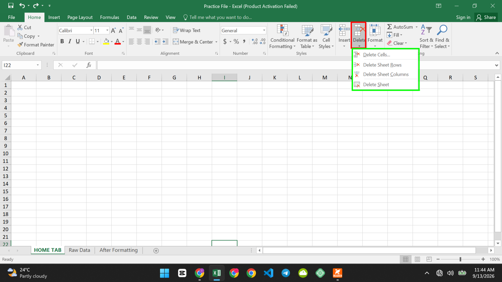
Delete: It removes a cell, row, column, or sheet.
Shortcut: Ctrl+- (minus sign).
Use case: removing a category you no longer track, like a subscription you canceled.
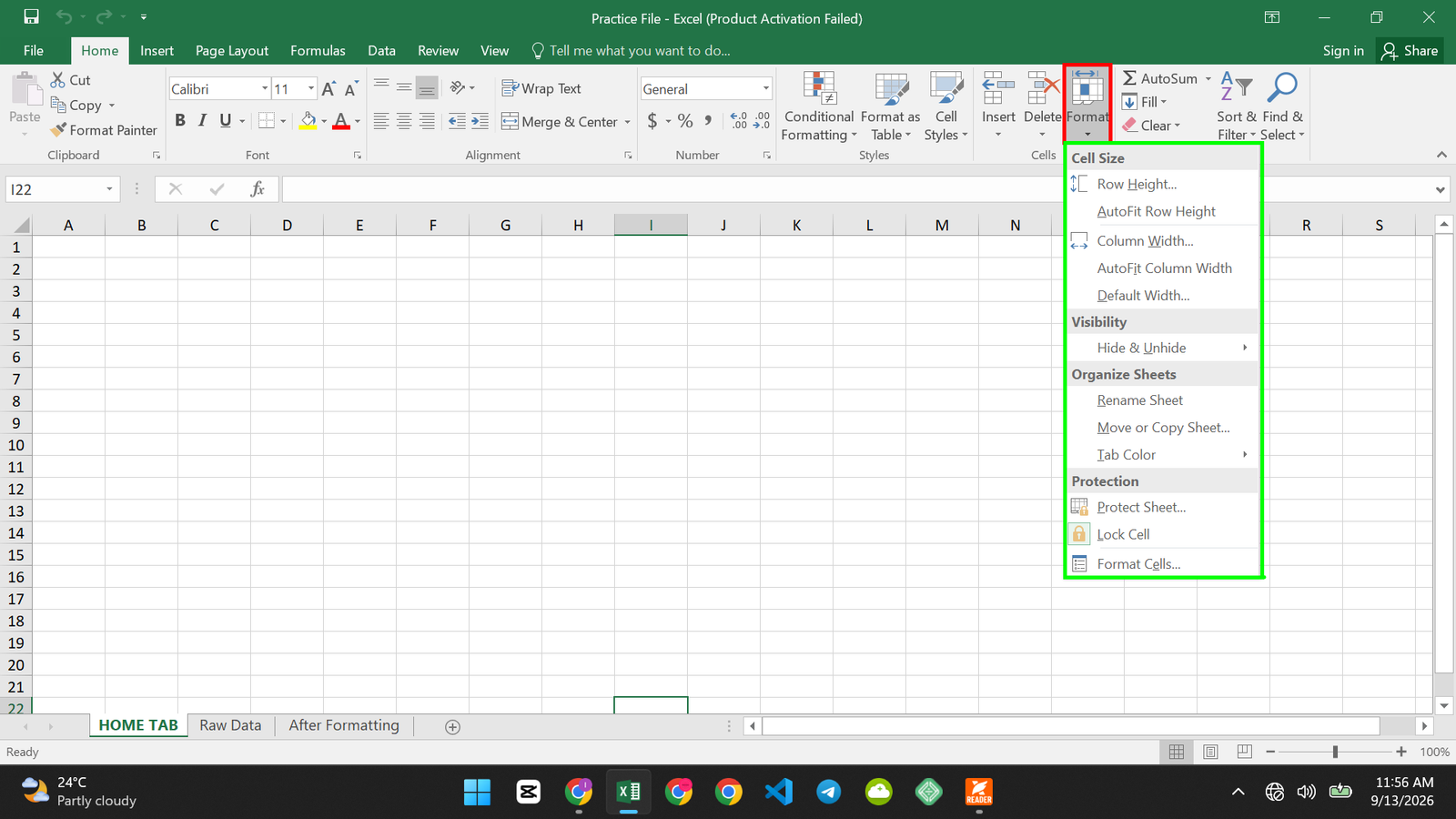
Format: It opens options for row height, column width, hiding or unhiding, and protecting cells. Shortcut: no default shortcut for the menu itself, but Alt, H, O opens it.
Use case: widening a column so a long tail word isn’t cut off.
Group 7: Editing
The last group, and one of the most useful for actually working with your numbers.
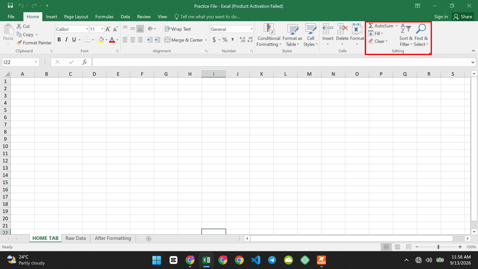
AutoSum: It guesses the range above or beside your cursor and writes a SUM, AVERAGE, MIN., MAX., ETC formula for you.
Shortcut: Alt+= (equals sign).
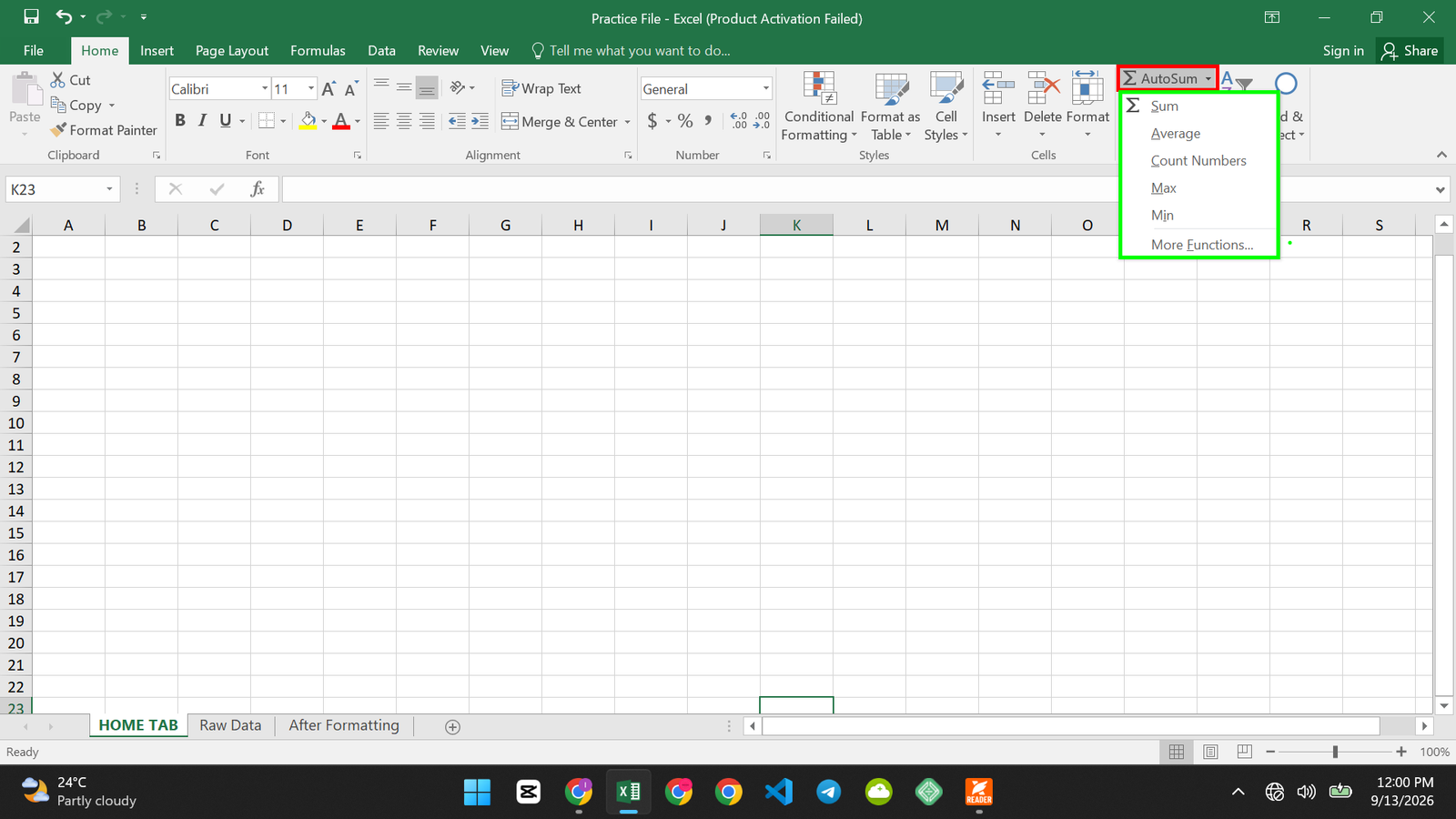
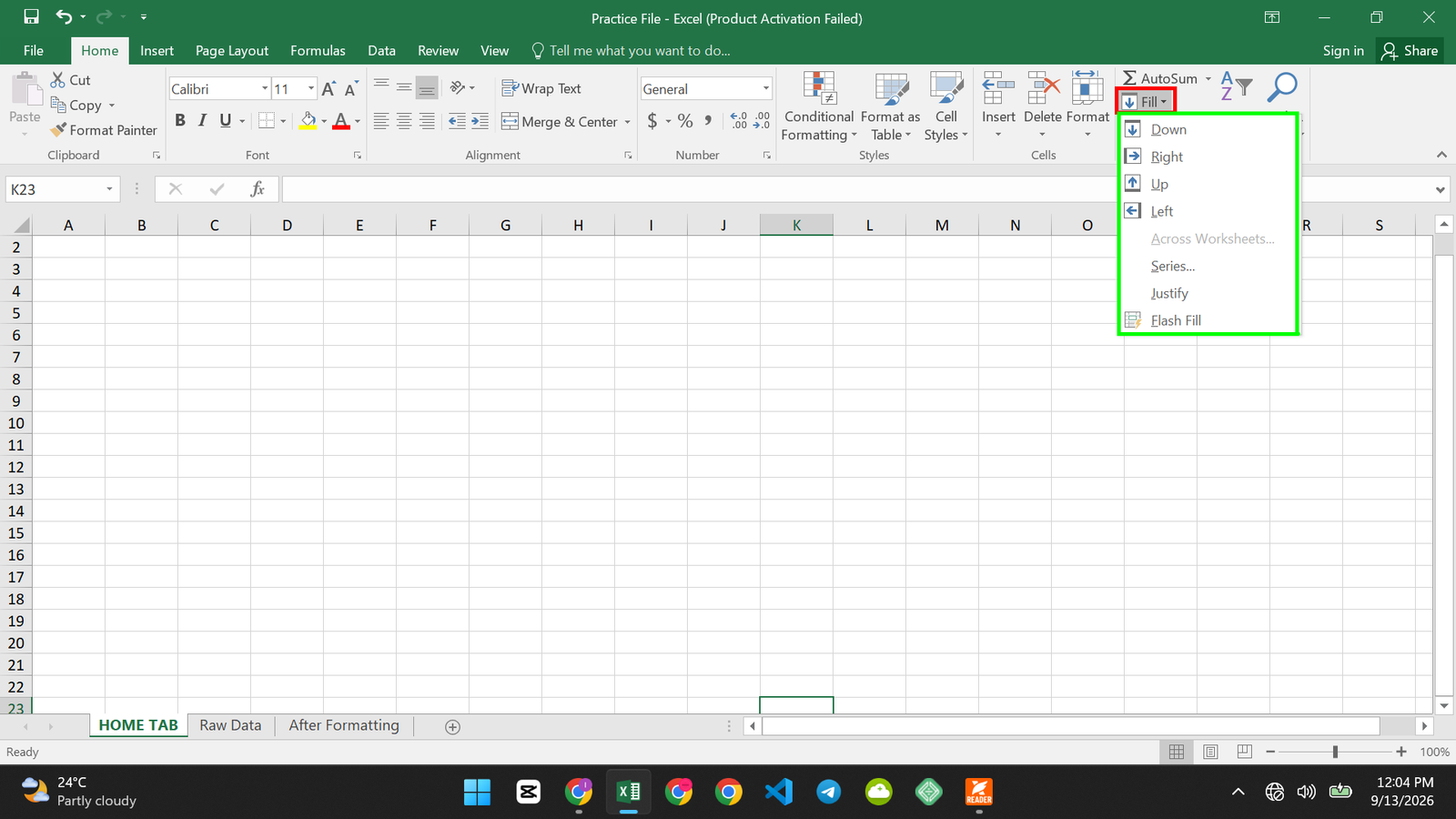
Fill: It copies a value or formula into adjacent cells, or continues a pattern.
Shortcut: Ctrl+D fills down, Ctrl+R fills right.
Use case: copying formula down through every row without dragging the fill handle by hand.
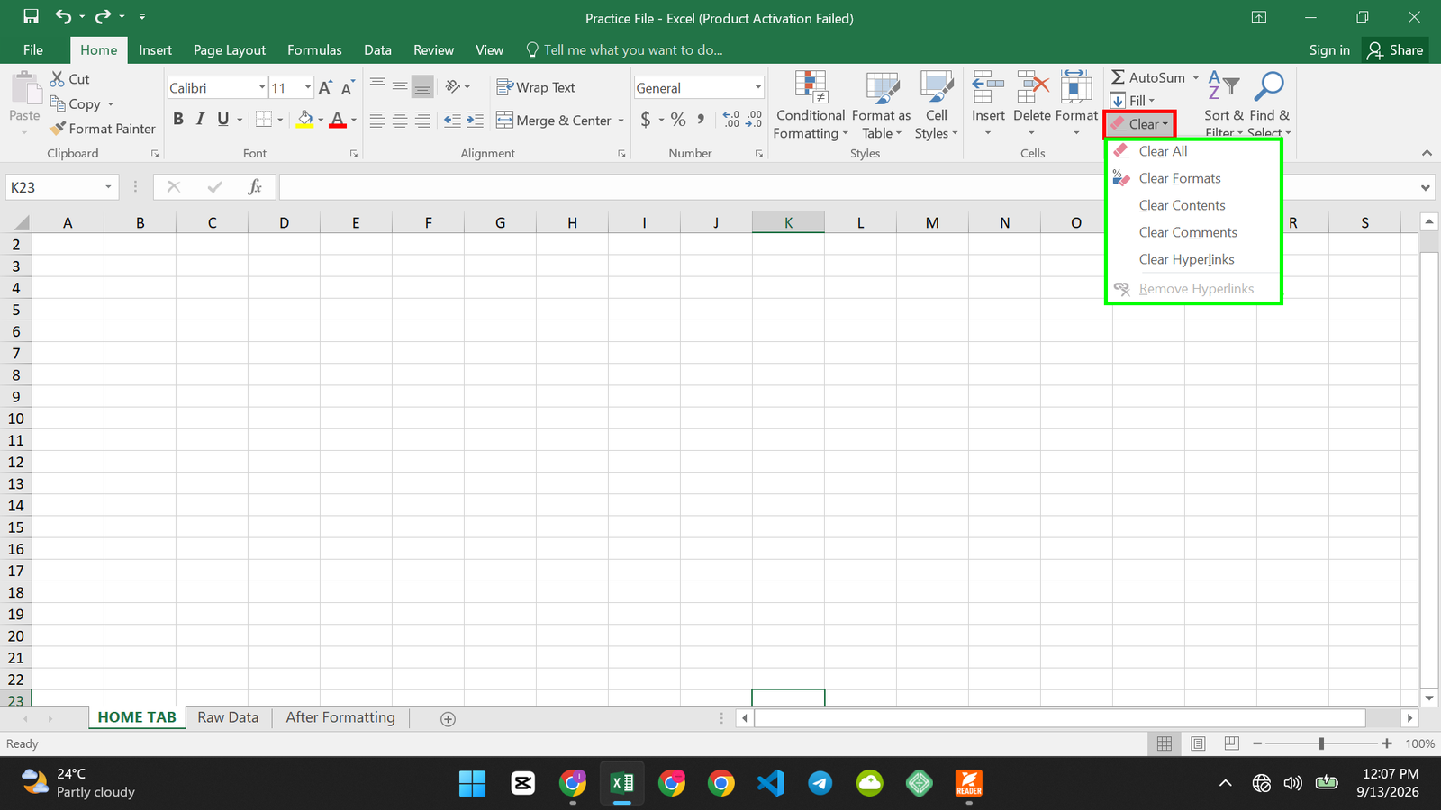
Clear: It removes contents, formatting, comments, or all three from selected cells.
Shortcut: the Delete key clears contents only, this button gives you more control.
Use case: wiping out a formula but keeping the cell’s formatting intact for reuse.
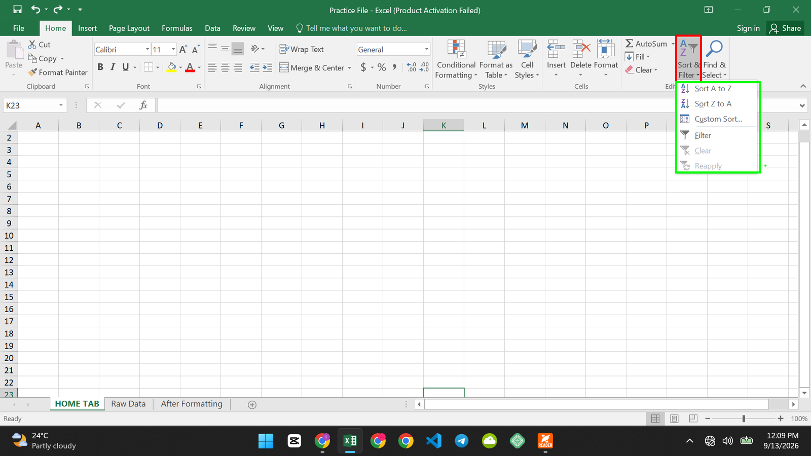
Sort & Filter: It reorders your data, or hides rows that don’t match a condition.
Shortcut: Ctrl+Shift+L toggles filter arrows on and off.
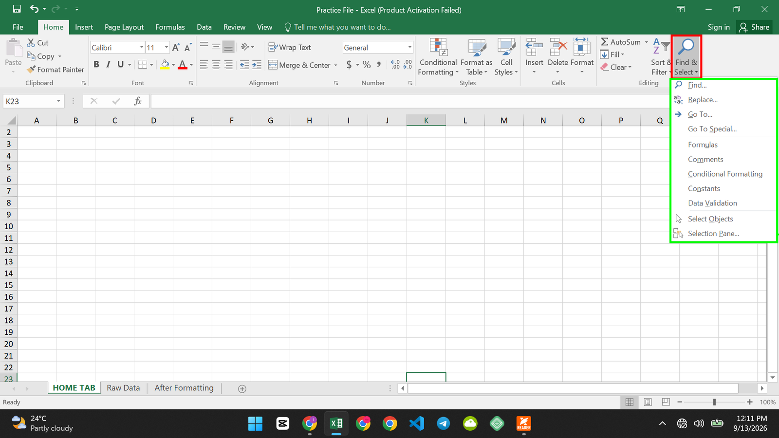
Find & Select: It locates specific text or values, replaces them, or jumps to special types of cells.
Shortcut: Ctrl+F for Find, Ctrl+H for Replace, Ctrl+G for Go To.
Use case: finding every cell that references a category you’re about to rename.
Why This Works
Every command on the Home tab either changes how your data looks or changes your data itself, and the groups are ordered roughly by how often you’ll reach for them. Clipboard and Font sit on the far left because you’ll touch them constantly. Cells and Editing sit further right because you’ll use them a little less often, but still all the time. Once you know a command by its group, you’ll find it fast, even in a version of Excel you’ve never opened before.
A Different Way to Do It
Almost everything on the Home tab also lives in a right-click menu.
Select a cell, right-click, and you’ll see Cut, Copy, Paste, and a Format Cells option that covers Font, Alignment, and Number all in one dialog box. I’d use the right-click menu when my hand is already on the mouse and I don’t want to reach up to the Ribbon, though learning the Ribbon layout is still worth it for the commands that aren’t in that menu, like Conditional Formatting.
Common Problems and How to Fix Them
| Problem | Why It Happens | How to Fix It |
| Bold or Italic won’t turn off | You selected a cell range where some cells are already bold and some aren’t, so clicking toggles them unevenly | Select just the cells you want, and click the button twice if needed to force it off everywhere |
| A number still shows as text after applying Number Format | The value was typed with an apostrophe or imported as text | Click the warning icon that appears, then choose Convert to Number, before applying the format |
| Merge & Center is grayed out | You’ve selected cells that are already part of a table or a protected sheet | Convert the range back to a normal range, or unprotect the sheet first |
| AutoSum picks the wrong range | It guessed based on nearby blank cells or a stray value | Adjust the highlighted range manually before pressing Enter |
Tips to Avoid These Problems Next Time
- Select your exact range before applying formatting, rather than a whole column, so you don’t accidentally affect cells you didn’t mean to.
- Check AutoSum’s suggested range before hitting Enter, it’s usually right, but not always.
- Use Format Painter instead of manually recreating formatting, it’s faster and keeps things consistent.
Frequently Asked Questions
What is the Home tab used for in Excel? It holds your most common formatting and editing tools: fonts, alignment, number formats, cell styles, and basic editing commands like AutoSum and Sort.
What are the seven groups on the Home tab? Clipboard, Font, Alignment, Number, Styles, Cells, and Editing, arranged left to right roughly by how often you’ll use them.
What is the shortcut for AutoSum? Alt and the equals sign (Alt+=). It writes a SUM formula based on the numbers around your selected cell.
How do I copy formatting without copying the data? Use Format Painter, in the Clipboard group. Click the cell with the formatting you want, click Format Painter, then click the cell you want to apply it to.
Why is my currency formatting not showing a dollar sign? You may have applied Comma Style instead of Accounting Number Format, they look similar but only one adds a currency symbol.
Wrapping Up
You now know every command on the Excel Home tab, what each one does, how to trigger it with a shortcut, and when you’d actually reach for it. That’s the tab you’ll open more than any other, so this knowledge pays off immediately. If you haven’t already, start with Excel Interface Explained: Ribbon, Toolbar, and Backstage View for Beginners